- Dimension Reduction
- Clustering
- Classification Performance
- Identifying Top Predictive Genes
- Conclusions
Dimension Reduction
Unsupervised
Applying PCA on the selected genetic features, the first component captured 65% of the variance in the data and the first 65 components captured 95% of the variance (Figure 1).
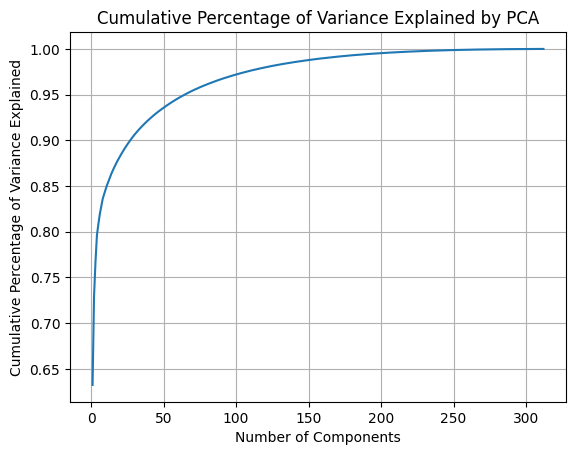
Figure 1: Cumulative percentage of variance explained by principal components.
Next, we visualized the first two principal components to assess their predictive power for the labels of interest. Figure 2 reveals that the cancer and healthy samples exhibit substantial overlap in the distribution of the two principal components, indicating that that these components may not be very informative for determining cancer status. Similarly, the two principal components were not informative of cancer stage (Figure 3).
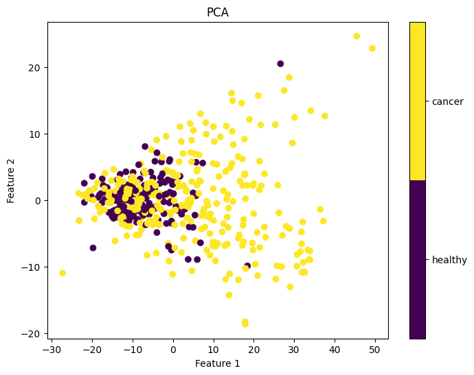
Figure 2: First two principal components colored by ground truth cancer status.
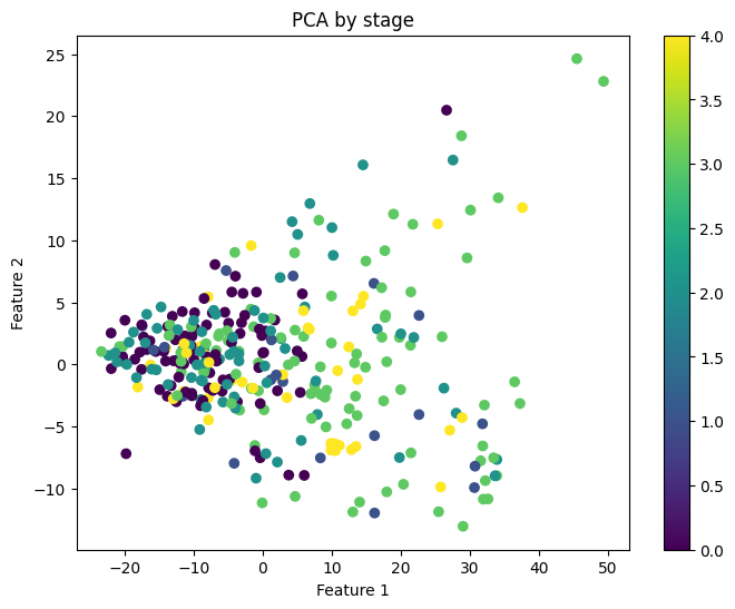
Figure 3: First two principal components colored by cancer stage.
The first two embedding dimensions obtained from unsupervised UMAP are shown in Figure 4. Similar to the PCA results, cancerous and healthy samples largely overlap, indicating that these embeddings are not informative of the cancer status either.
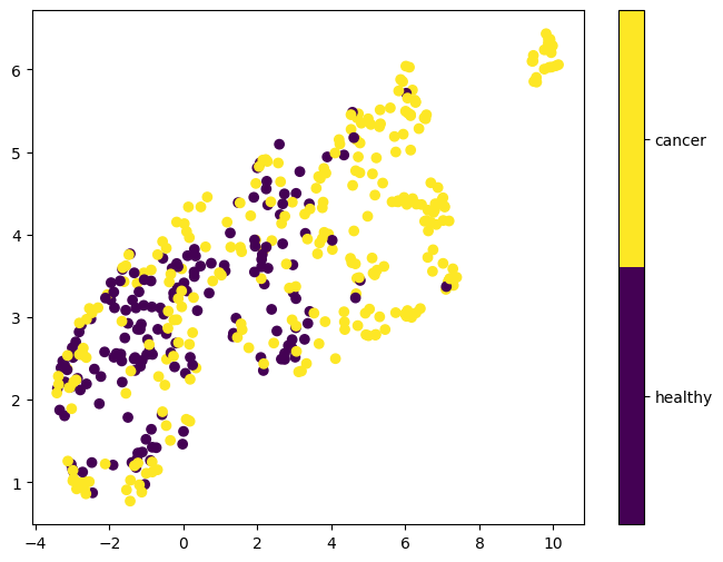
Figure 4: First two UMAP embeddings after unsupervised UMAP dimensionality reduction
The unsupervised PCA and UMAP results suggest that unsupervised dimension reduction, linear or non-linear, cannot extract predicitve informative features from this dataset. This is likely because the signal in genetic data is typically sparse coupled with measurement noise.
Supervised
To obtain more informative components, we applied supervised UMAP, which uses the label to learn a lower-dimensional space to preserve not only the intrinsic geometric structure of the data but also the class-level relationships. As shown in Figure 5, supervised UMAP generated embeddings that can separate cancerous and healthy samples very well.
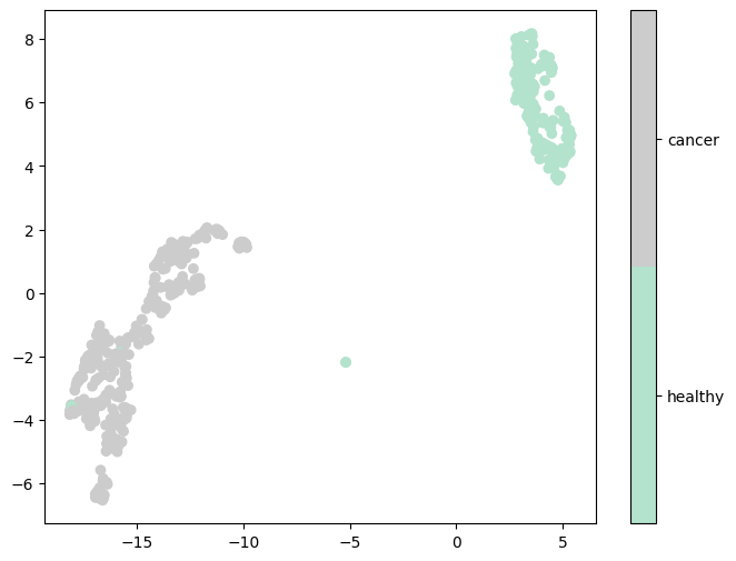
Figure 5: First two UMAP embeddings after supervised UMAP dimensionality reduction based on cancer status.
We are also interested in assessing the informativeness of embeddings in identifying the origin of cancer. We applied supervised UMAP on cancerous samples, treating cancer type as a categorical label. Results show that the resulting UMAP embeddings are distributed in separable clusters, suggesting that they will be informative predictors for cancer type classification (Figure 6).
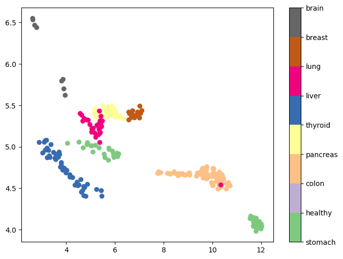
Figure 6: First two UMAP embeddings after supervised UMAP dimensionality reduction based on cancer type.
Later analysis showed that using UMAP embeddings as input to the classification models achieved perfect accuracy on the training set but poor accuracy on the test set, suggesting that UMAP embeddings are prone to overfitting. In contrast, PLS components achieved much better test accuracy in classification tasks even though they don’t provide visual separation of classes.
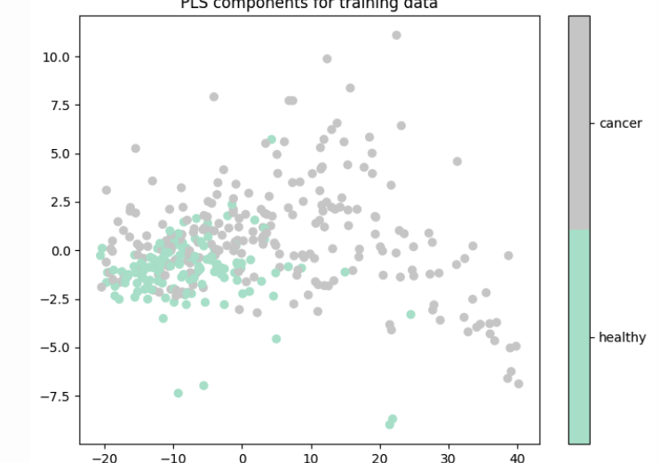
Figure 7: First two PLS components based on cancer status of training data.
Clustering
Using the UMAP embeddings as input features, clustering algorithms were able to achieve high ARI and NMI when compared to the ground truth cancer type. The best performing clustering algorithm was DBSCAN, likely due to it’s capability to handle clusters of varying shapes, sizes, and densities, which is an inherent characteristic of our data from different types of cancer. These positive clustering results imply promising prospects for developing accurate cancer detection and cancer classification models using cfDNA data.
| Method | ARI | NMI |
|---|---|---|
| K-Means | 0.91 | 0.95 |
| Hierarchical Clustering | 0.84 | 0.91 |
| DBSCAN | 0.92 | 0.95 |
| Gaussian Mixture Models | 0.70 | 0.86 |
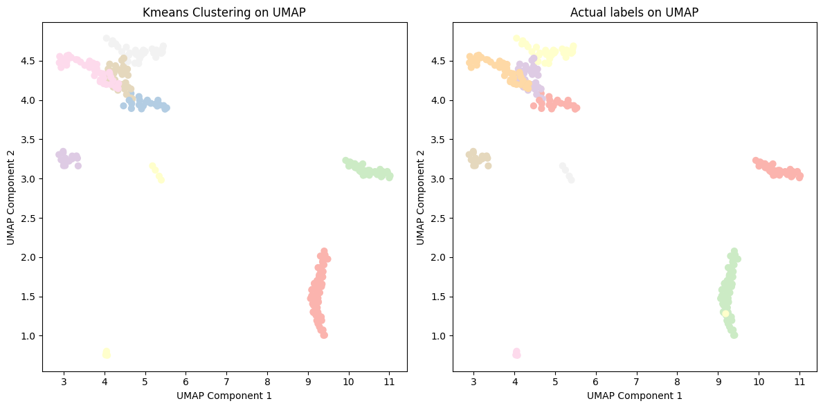
Figure 9: Kmeans clustering of cancer type with UMAP embeddings.
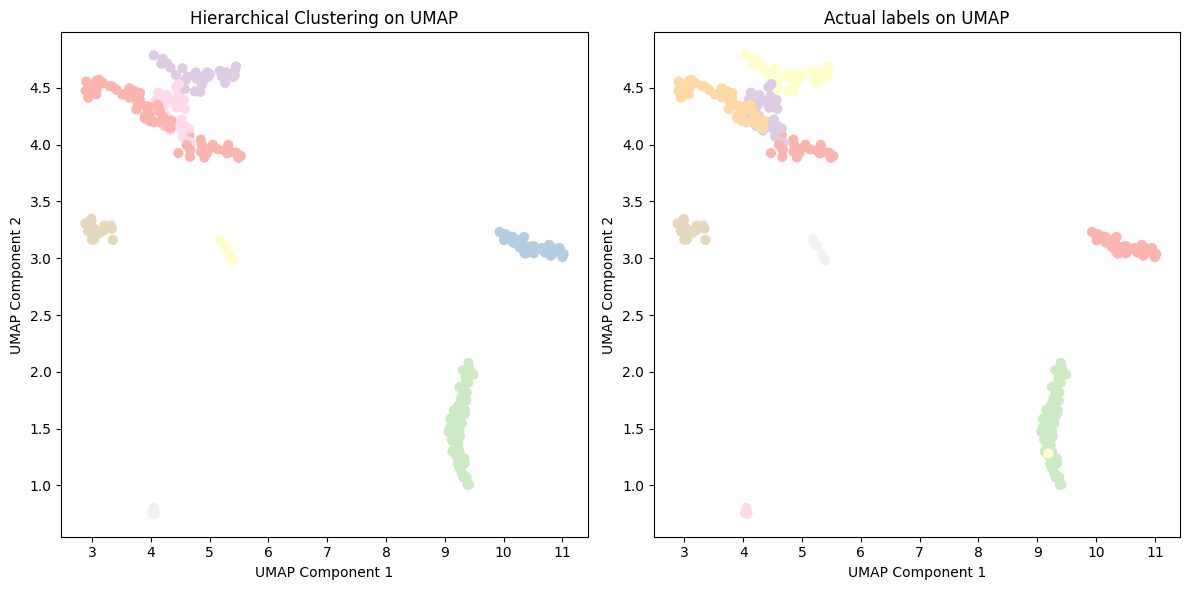
Figure 10: Hierarchical clustering of cancer type with UMAP embeddings.
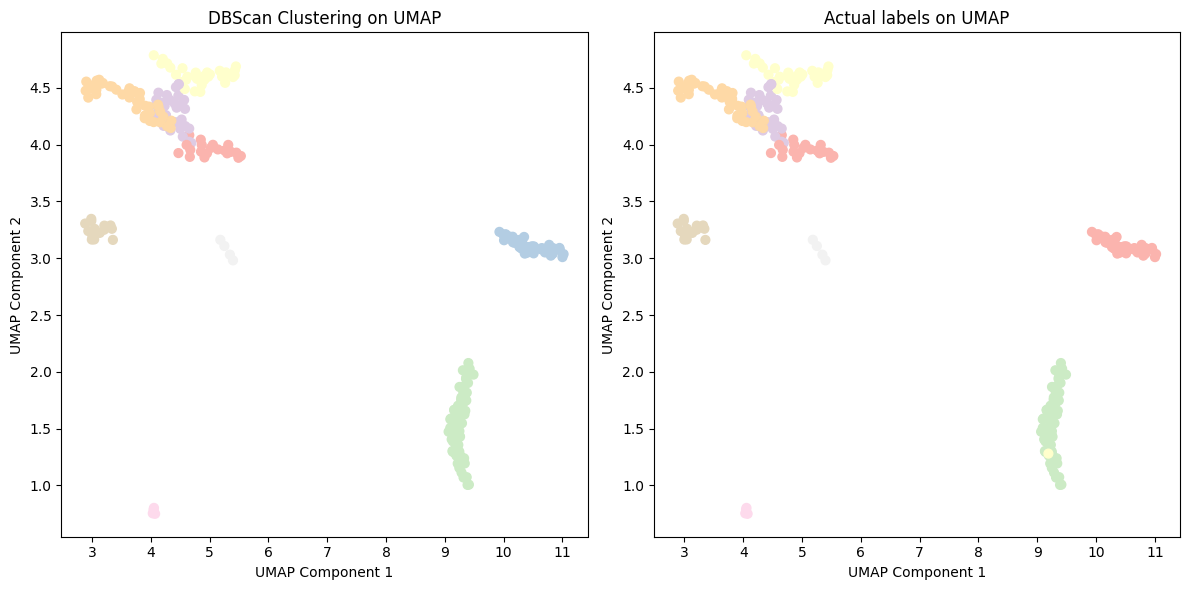
Figure 11: DBSCAN clustering of cancer type with UMAP embeddings.
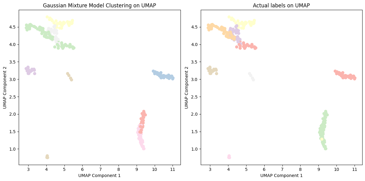
Figure 12: GMM clustering of cancer type with UMAP embeddings.
Classification Performance
There are two steps to our model evaluation. First, how accurate can our models detect cancer from a cfDNA sample. Second, if a sample is detected to be cancerous, how accurate can our models detect the tissue of origin of the cancer, i.e. classify the cancer type.
Cancer Detection
The cancer detection results based on random train test split are shown in Table 1. The best models achieved approximately 0.854 AUC in cancer detection. Note that we focus on using AUC to discuss model performance as the accuracy metric can be affected by sample imbalance and is dependent on the thresholding of the probabilistic predictions.
Table 1: Results of cancer detection (random train-test split).
| Feature Selection | Classifier | Num PLS Components | Test Accuracy | Test AUC |
|---|---|---|---|---|
| Univariate | Random Forest | 6 | 0.737 | 0.841 |
| Logistic Regression | 6 | 0.737 | 0.824 | |
| Differential Gene Expression | Random Forest | 4 | 0.768 | 0.854 |
| Logistic Regression | 4 | 0.789 | 0.841 |
In addition, we summarize results when models are trained using data from one study and evaluated on an independent test set from another study in Table 2. We observed that test AUC significantly decreased to 0.688. These results suggest that despite our models have reasonably good cancer detection performance from previous results, they do not generalize well across studies.
Table 2: Results of cancer detection(train-test split by study).
| Feature Selection | Classifier | Num PLS Components | Test Accuracy | Test AUC |
|---|---|---|---|---|
| Univariate | Random Forest | 5 | 0.656 | 0.688 |
| Logistic Regression | 5 | 0.623 | 0.522 | |
| Differential Gene Expression | Random Forest | 4 | 0.754 | 0.653 |
| Logistic Regression | 4 | 0.705 | 0.633 |
Sequential Cancer Type Classification
Mean AUC results between models with PLS components based on univariate feature selection versus differential gene expression (DE) feature selection suggested that the DE feature selection method resulted in slightly better classification (Figure 13). Selecting genes via DE achieved better performance for colon, stomach, thyroid; and univariate feature selection had better performance for pancreas and liver cancers (Figure 13). Considering that DE significantly improved the performance of the worst performing thyroid cancer detection model, we chose DE as the preferred method.
Between Random Forest and Logistic Regression classifiers, Random Forest classifiers performed slightly better, with a mean AUC of 0.777 across cancer types and class weight augmentation methods versus 0.756 for Logistic Regression (Figure 14). Classifier model type (Random Forest/Logistic Regression) varied by cancer type with regard to which model performed better. For detecting colon and stomach cancers, Logistic Regression’s performance was on par with Random Forest. For detecting pancreas and liver cancers, Logistic Regression outperformed Random Forest. However, Logistic Regression had poor performance for detecting thyroid, significantly worse than Random Forest. It is worth noting that the later three cancer types (thyroid, pancreas, liver) had a smaller sample size, thus the results may fluctuate across different train/test splits. Logistic Regression is a simpler, more robust classifier in small sample size cases .
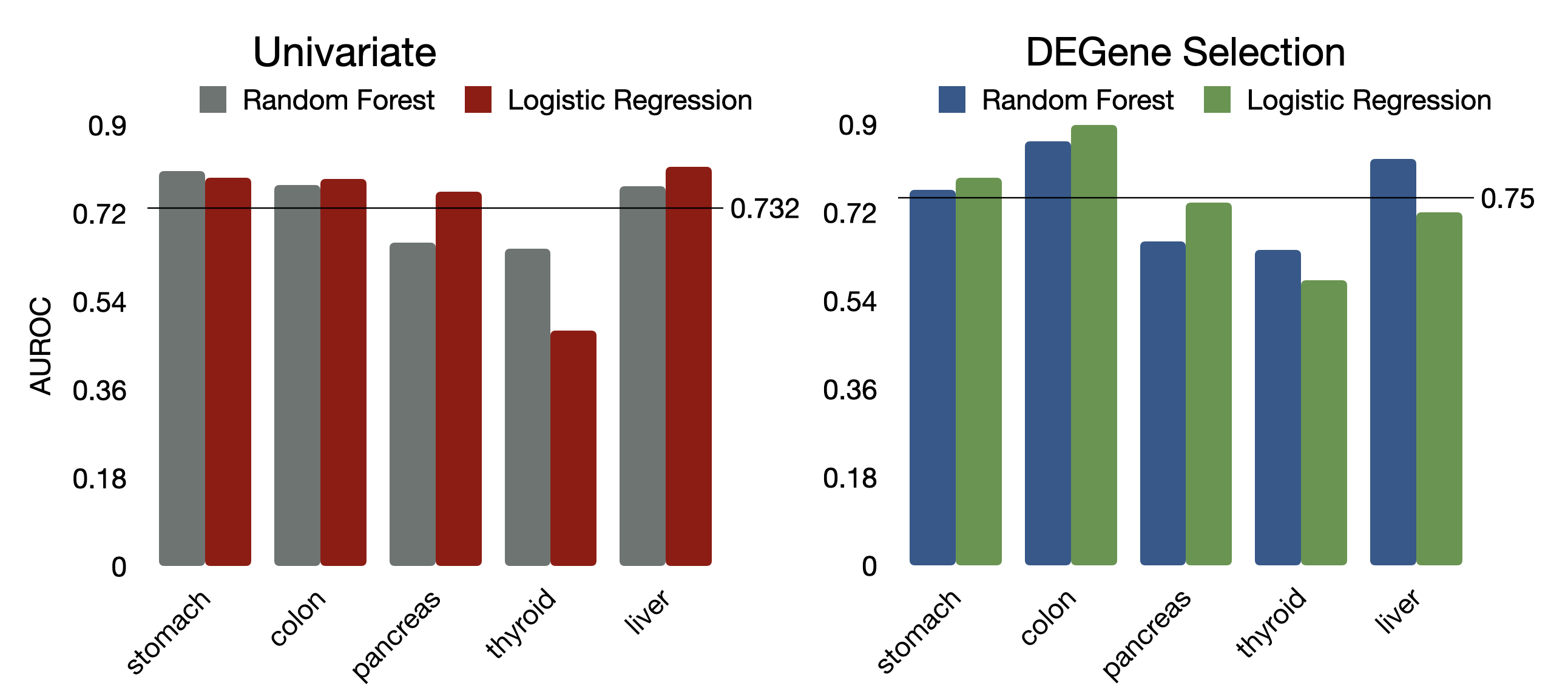
Figure 13: Area under the ROC curve values by feature selection type.
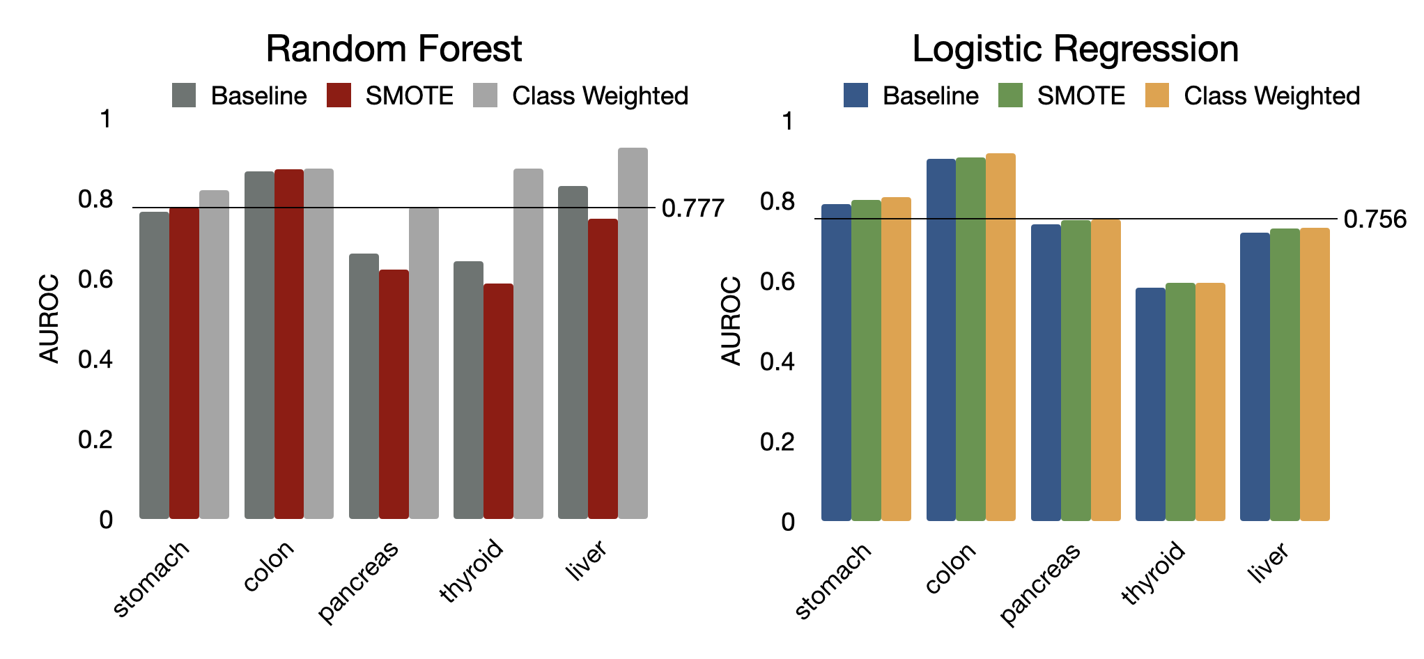
Figure 14: Area under the ROC curve values by class weight augmentation and classifier model type.
When using train test split by study, the cancer type classification performance is significantly worse compared to using random train/test split from the combined dataset (Figure 15).

Figure 15: Results of cancer type classification (train-test split by study). Note that thyroid cancer could not be evaluated because this cancer did not have any data in one of the studies.
Identifying Top Predictive Genes
We examined the feature contribution of each gene in the best performing model discussed in the previous section (Logistic Regression + DE + class weights). Interestingly, some top predictive genes are shared across multiple cancers, whereas others are specific to each cancer (Figure 16).
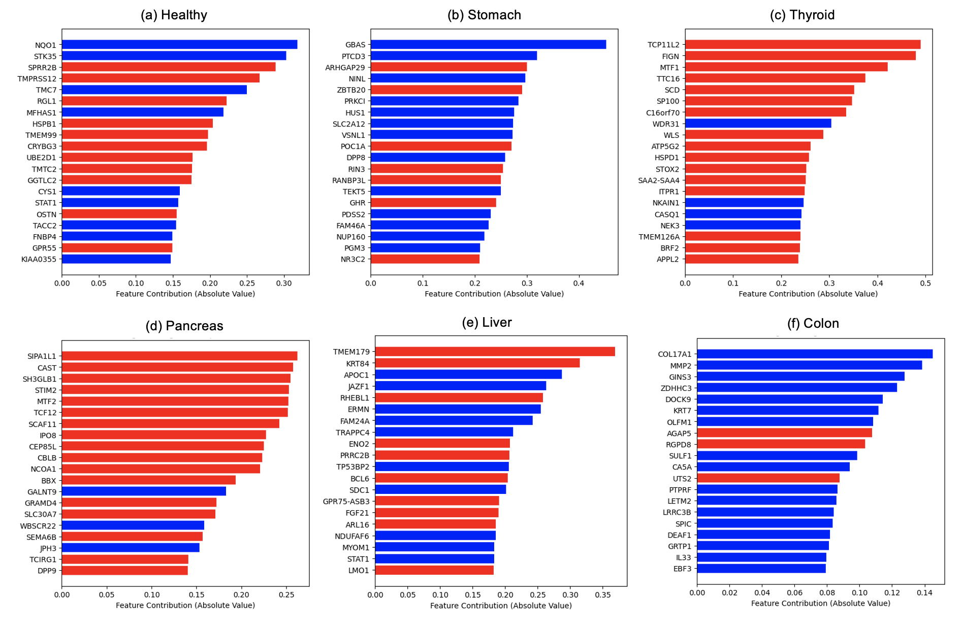
Figure 16: Top contributing genes to each classification model. Blue: contributing in the positive direction with respect to class 1; Red: contributing in the negative direction with respect to class 1.
Conclusions
This project examined the utility of 5-hmc cfDNA data for cancer diagnostics using machine learning. We developed a two-step classification pipeline that consisted of first a cancer detection model (healthy vs. cancerous) followed by a cancer origin classification model (cancer type). To tackle the high-dimensionality of the data coupled with relatively small sample size, multiple feature selection methods, dimension reduction techniques, classifiers, and strategies to tackle data imbalanced were explored and compared. Methods were developed and evaluated using data from two independent studies that encompassed nine cancer types. The best performing models achieved 0.854 AUC for cancer detection and 0.600 - 0.920 AUC for detecting different types of cancers, with excellent detection performance for colon cancer, good performance for stomach, pancreas, and liver cancers, and poor performance for thyroid cancer. However, the generalization capability of these models to independent test datasets obtained from different data collection centers is poor.
Next steps
- This analytical pipeline should be run with multiple seeds to check precision in classification performance.
- The predictive classification performance from the study dataset split were relatively poor compared to the balanced dataset split results. This suggests we need a larger training dataset across multiple studies to account for batch effects.
- We would also like to add additional gene expression data from samples associated with other diseases to ensure that our classification of cancer versus healthy is specific to cancer versus disease (and immune response to disease) in general